A practical framework for building timeframe-specific models that respond dynamically to shifting market conditions
In our previous article, Regime Changes and Market Microstructure, we examined how market regimes manifest differently across timeframes – from tick-level microstructure dynamics to macro weekly cycles – and how each transition leaves a distinct fingerprint in order flow, liquidity, and price behavior.
The natural next question is: how do you actually build models around this?
Understanding that regimes exist is only the first step. The real challenge is engineering systems capable of detecting changing market conditions in real time, translating those conditions into actionable strategy logic, and aligning signals across multiple timeframes.
This article presents the Adaptive Regime Framework — a production-oriented market intelligence architecture designed to combine:
- Real-time order book liquidity
- Market microstructure analytics
- Cross-asset pricing intelligence
- AI-driven news sentiment
- Multi-timeframe regime detection
- Adaptive risk management
Instead of relying on a single universal trading model, the framework treats every timeframe as its own behavioral environment, powered by its own market drivers, data sources, and regime logic.
The result is a fully adaptive trading architecture capable of responding dynamically to changing liquidity conditions, volatility environments, macroeconomic shifts, and market narratives.
Why the universal regime models fail
One of the most common mistakes in quantitative trading is attempting to build a single regime model and apply it across all timeframes.
The intuition is understandable: One model. One signal. One source of truth.
In practice, this approach fails because the drivers of market behavior change completely as you move across the timeframe hierarchy.
At the tick level, market behavior is dominated by:
- Order book imbalance
- Liquidity depletion
- Spread dynamics
- Trade arrival rates
- Informed vs. uninformed flow
At the weekly or monthly level, regimes are governed by:
- Central bank policy
- Credit conditions
- Inflation expectations
- Liquidity cycles
- Macroeconomic narratives
A model designed for one environment becomes structurally blind to the dynamics of another.
The Adaptive Regime Framework solves this problem through a layered architecture where:
- Each timeframe receives its own regime model
- Each model uses timeframe-specific feature sets
- Each layer is powered by dedicated Jungletrade market intelligence products
- All layers are synthesized through cross-timeframe alignment
The Jungletrade Market Intelligence Stack
For the purpose of the article we are using Jungletrade market intelligence infrastructure.
Each Jungletrade product contributes a different layer of market awareness.
- Spot Order Book – High-frequency order book liquidity and depth analytics data that combines multiple centralized exchanges.
- Spot Liquidity Walls – High-impact liquidity walls and significant support/resistance price levels.
- Crypto Spot Prices Flow – Real-time cryptocurrency pricing
- FX Exchange Rates – Global currency pressure and macro direction
- News Sentiment (MENTIS) – AI-powered market sentiment intelligence analyzing financial news, media narratives, and market commentary in real time.
- Market Condition Model (OMNIS) – AI-powered market condition model aggregating weighted financial, macroeconomic, and geopolitical news sentiment over the past 6 hours using impact scoring and time-decay analysis.
The Core Model Toolkit
Rather than relying on a single statistical methodology, the system uses different models depending on the behavioral characteristics of each timeframe.
1. Hidden Markov Models (HMM)
HMMs assume the market transitions between a finite number of hidden states that are not directly observable but produce observable outputs, such as:
- Returns
- Volatility
- Volume
- Liquidity imbalance
- Spread behavior.
Best suited for: Identifying regimes purely from price and volume time series, across any timeframe. The “hidden” aspect is a strength here, you are not imposing regime labels, you are discovering them from the data.
Key advantage: Regimes discovery directly from the data rather than imposing predefined labels.
2. Markov-Switching Autoregression (MS-AR)
MS-AR models extend HMMs by allowing the autoregressive structure of returns to switch between regimes.
This enables the model to capture:
- Momentum persistence
- Mean reversion
- Volatility clustering
- Regime-dependent autocorrelation
Best suited for: Daily and weekly timeframe analysis where autocorrelation structure is meaningful and regimes tend to persist for multiple periods.
3. Threshold Models (SETAR / STAR)
Threshold models switch regimes when observable market variables cross predefined boundaries.
Examples include:
- Liquidity imbalance thresholds
- Volatility expansion
- Hurst exponent transitions
- News sentiment pressure scores
- VIX regime boundaries
These models are highly interpretable and suitable for structural regime transitions.
Best suited for: Structural regime transitions.
4. Hybrid Ensemble Models
Modern production systems typically combine statistical regime detection (HMM or MS-AR) with supervised machine learning (gradient boosted trees, LSTM networks) trained on labeled historical regimes. The statistical model provides the regime probability framework; the ML layer sharpens it using a richer feature set.
The model may combine:
- Statistical regime models
- Machine learning classifiers
- Liquidity intelligence
- News sentiment analytics
- Cross-timeframe alignment
Best suited for: Combined approach where Statistical models establish regime probabilities and the Machine learning layers refine those probabilities using richer feature sets.
JungleTrade Market Microstructure Regime Model
1. Tick / Sub-Minute — Microstructure Regime Models
At the tick level, regime detection is entirely an order flow problem. Price formation here is dominated by the interaction between informed and uninformed participants, and the regime shifts occur in seconds — well before they become visible on any candlestick chart.
This layer is powered primarily by:
- Spot Order Book
- Spot Liquidity Walls
- Crypto Spot Prices Flow
The key objective is to identify:
- Informed directional flow
- Liquidity exhaustion
- Spread instability
- Liquidity crises
- Execution risk
The three states to model at this level:
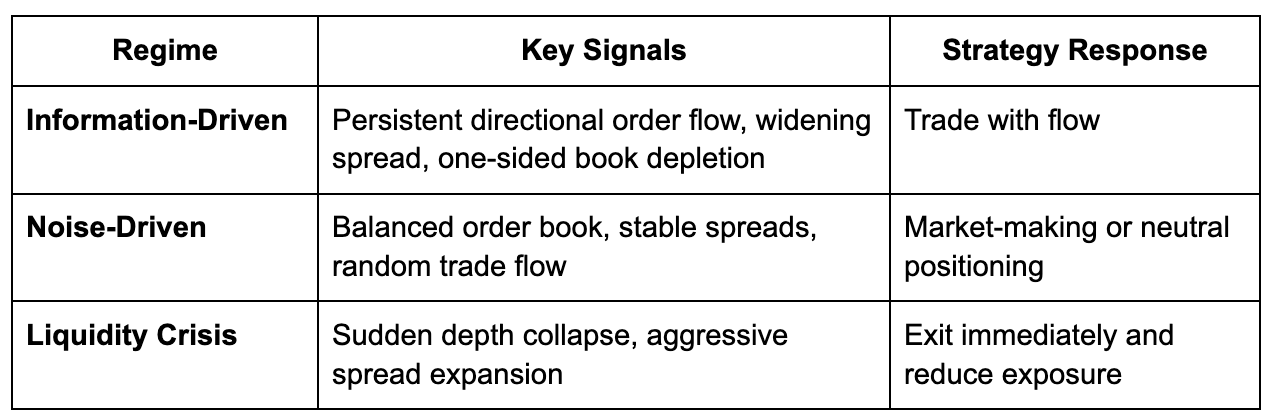
Feature inputs:
- Top-level order book imbalance
- Bid/ask liquidity concentration
- Liquidity wall formation
- Spread Z-score expansion
- Trade arrival acceleration
- Real-time depth depletion analysis
Model architecture:
- Spot Order Book provides the raw liquidity states
- Spot Liquidity Walls identifies significant liquidity concentrations and support/resistance structures.
- Crypto Spot Prices Flow provides real-time pricing and spread normalization.
- The model continuously updates regime probabilities on every new market update.
- Latency becomes a critical engineering constraint — a correct model that reacts too slowly is functionally useless at the microstructure level.
2. 1-Minute to 5-Minute – Intraday Momentum Regime Models
At the 1–5 minute level, regimes reflect the interplay of session structure, news impact, and institutional order absorption. A critical insight from our microstructure analysis is that markets display strong intraday seasonality — the 9:30–10:00 am regime is structurally different from the 12:00–2:00 pm regime, even if the raw price action looks similar on both.
At the intraday timeframe, market behavior begins reflecting:
- Session structure
- Institutional order absorption
- News-driven volatility
- Liquidity concentration shifts
This model layer integrates:
- Crypto Spot Prices Flow
- Spot Order Book
- Spot Liquidity Walls
- News Sentiment (MENTIS)
The four states to model at this level:
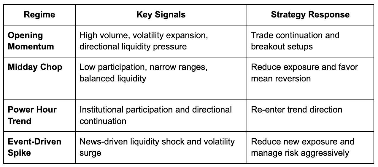
Feature inputs:
- Session-normalized volatility
- VWAP deviation
- Volume acceleration
- Liquidity imbalance persistence
- News sentiment pressure score
- Intraday liquidity concentration changes
Model architecture:
News Sentiment (MENTIS) becomes particularly important at this layer.
The model evaluates how recent financial, macroeconomic, and geopolitical narratives influence intraday liquidity conditions.
AI-driven sentiment scoring is combined with order book structure to distinguish genuine directional expansion from temporary volatility noise.
3. 15-Minute to 1-Hour — Intraday Structural Regime Models
At this timeframe, market microstructure begins to smooth out. What remains are structural elements: support and resistance zones, VWAP bands, hourly pivot levels, and the order block structures that institutional participants defend. As noted in our previous article, institutional order flow consistently respects hourly levels, making this the most reliable timeframe for identifying intraday inflection points.
The dominant drivers become:
- Structural liquidity zones
- Liquidity-based support and resistance
- Compression and breakout structures
- Institutional participation
This layer is primarily powered by:
- Crypto Spot Prices Flow
- Spot Liquidity Walls
- CryptoQuote
- Market Condition Model (OMNIS)
- Regime Persistence Index (RPI)
The four states to model at this level:
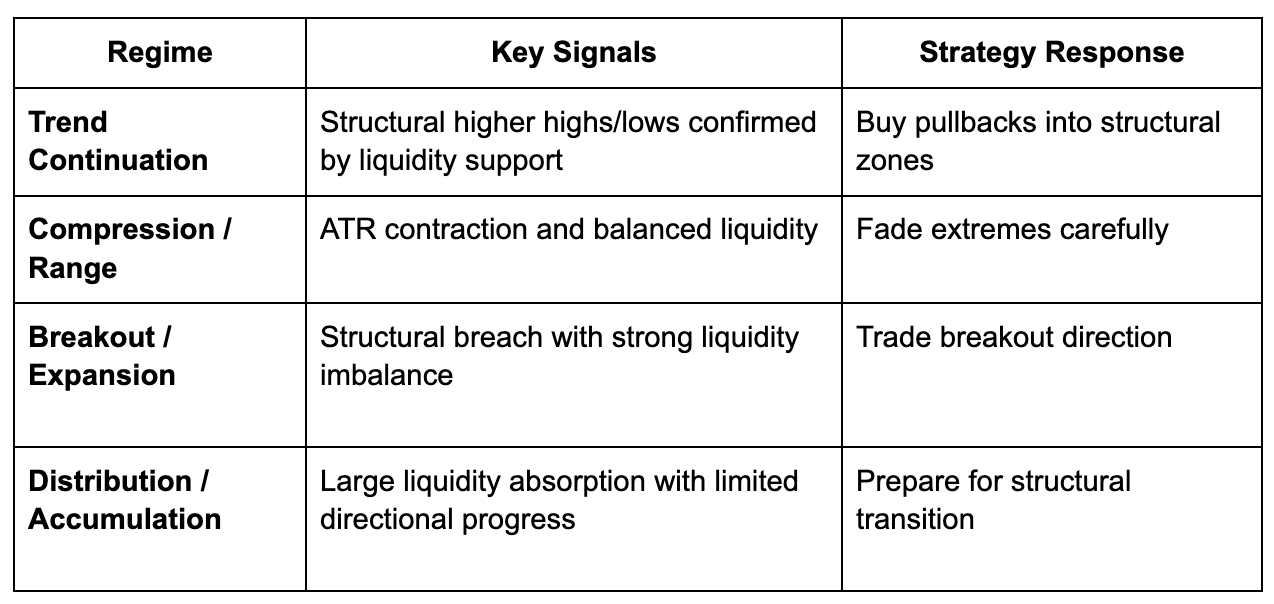
Feature inputs:
- Liquidity-based support/resistance strength
- Hurst exponent regime classification
- ATR expansion ratio
- Structural breakout detection
- Liquidity wall absorption
- Volume-weighted order flow direction
Model architecture:
Spot Liquidity Walls becomes the dominant intelligence layer at this timeframe.
Rather than treating support and resistance as static price lines, the framework evaluates them dynamically using:
- Liquidity concentrations
- Order book pressure
- Depth persistence
- Liquidity wall formation
- Structural breakout probability
This creates adaptive support/resistance detection rather than traditional indicator-based levels.
The Market Condition Model (OMNIS) provides the necessary information about the news feed impact on human reactions and the transition of these reactions to the market behaviour.
The Regime Persistence Index helps us identify the transition probability between different market regimes.
4. 4-Hour — Swing Regime Models
The 4-hour chart is the canonical timeframe for swing trading. Regimes here typically persist 1–3 trading days, making them actionable for positions held from several hours to several days. At this resolution, daily fundamentals begin to seep into price, but short-term noise is still substantially filtered.
At this resolution:
- Short-term noise is filtered
- Structural trends become clearer
- Macro influence begins interacting with technical behavior
This layer combines:
- Crypto Spot Prices Flow
- FX Exchange Rates
- Market Condition Model (OMNIS)
- Structural Regime Engine (SRE)
- Inflation Rates
The four states to model at this level:
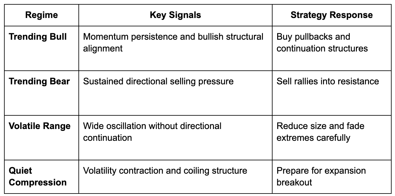
Feature inputs:
- EMA structural alignment
- Momentum persistence metrics
- Bollinger Band compression
- Realized volatility state
- FX directional pressure
- Precious metals defensive flow behavior
- Macro sentiment pressure
- Regime change probability
Model architecture:
At this layer, the framework begins incorporating cross-market intelligence.
- Crypto Spot Prices Flow
- FX Exchange Rates provide macro currency pressure.
- Structural Regime Engine provides the transition probabilities between different regimes and cycles.
- Market Condition Model (OMNIS) – provides the impact of the news flow to the margaret conditions and regimes and adds an additional narrative context influencing medium-term directional persistence.
- Inflation Rates provide additional information on the market sentiment structure. Usually people are protecting their funds from high inflation risk.
- Structural Regime Engine (SRE) – Detects the possible regime change.
5. Daily — Multi-Day Regime Models
At the daily timeframe, fundamental regime drivers take center stage: central bank policy, earnings cycles, credit conditions, and cross-asset correlations. Daily regimes tend to persist for weeks, and their transitions — while often visible in retrospect — carry substantial uncertainty in real time. This demands a more conservative model design with higher confidence thresholds before acting.
This layer is powered by:
- Market Condition Model (OMNIS)
- Regime Persistence Index (RPI)
- Structural Regime Engine (SRE)
- Crypto Spot Prices Flow
- FX Exchange Rates
- Spot Liquidity Walls
- Macro Data
The four states to model at this level:
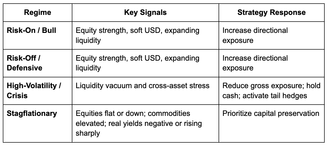
Feature inputs:
- FX directional strength
- Cross-asset correlation stress
- News sentiment pressure
- Volatility regime shifts
- Macro narrative persistence
Model architecture:
Regime Persistence Index (RPI), Market Condition Model (OMNIS) and Structural Regime Engine (SRE) become a central driver at this layer.
The model aggregates:
- Financial news
- Macroeconomic releases
- Geopolitical developments
- Cross-market narratives
The model aggregates:
- Financial news
- Macroeconomic releases
- Geopolitical developments
- Cross-market narratives
This creates a continuously updating market condition engine capable of measuring directional information pressure in real time.
Cross-Timeframe Alignment — The Cascade Framework
The most powerful feature of the Adaptive Regime Framework is cross-timeframe alignment.
Higher time frame regimes establish the structural context for lower time frame execution.
A strong lower timeframe signal that conflicts with the dominant higher timeframe regime is treated with skepticism and reduced sizing.
The Cascade Hierarchy
Daily Market Condition Regime ↓ 4H Swing Regime ↓ 1H Structural Liquidity Regime ↓ Intraday Liquidity Execution ↓ Tick-Level Microstructure Execution
The Alignment Score
The framework computes a weighted alignment score across all active regime layers.
Higher timeframe models receive larger weighting because they define broader structural conditions.
Strong alignment across multiple timeframes allows:
- Increased position size
- Higher conviction
- Wider stop placement
- More aggressive trend participation
Regime disagreement automatically reduces:
- Position sizing
- Trade frequency
- Directional conviction
This prevents one of the most common trading failures:
- Taking strong short-term signals directly against dominant macro conditions.
The Model Development Workflow
Building production-grade adaptive systems requires a disciplined development process.
Step 1: Regime Labeling
Historical regimes are initially identified using:
- Volatility clustering
- Trend persistence
- Liquidity conditions
- Cross-asset relationships
- News sentiment pressure
Step 2: Feature Engineering
The framework extracts normalized and stationary features from:
- Market depth
- Liquidity concentration
- Cross-asset pricing
- Volatility structure
- AI-driven sentiment analysis
Step 3: Model Training and Selection
Candidate models are evaluated based on:
- Out-of-sample accuracy
- Transition stability
- False positive rate
- Detection latency
- Regime persistence
Walk-forward validation is mandatory.
Static in-sample validation is insufficient for regime systems.
Step 4: Strategy Integration
Every detected regime maps directly into:
- Position sizing
- Entry aggressiveness
- Stop-loss logic
- Profit-taking methodology
- Risk exposure
The framework adapts trading behavior dynamically rather than applying static rules across all market conditions.
Step 5: Continuous Monitoring and Recalibration
Markets evolve continuously.
The framework therefore includes:
- Rolling retraining
- Regime drift monitoring
- Transition uncertainty alerts
- Liquidity structure recalibration
- Sentiment model updates
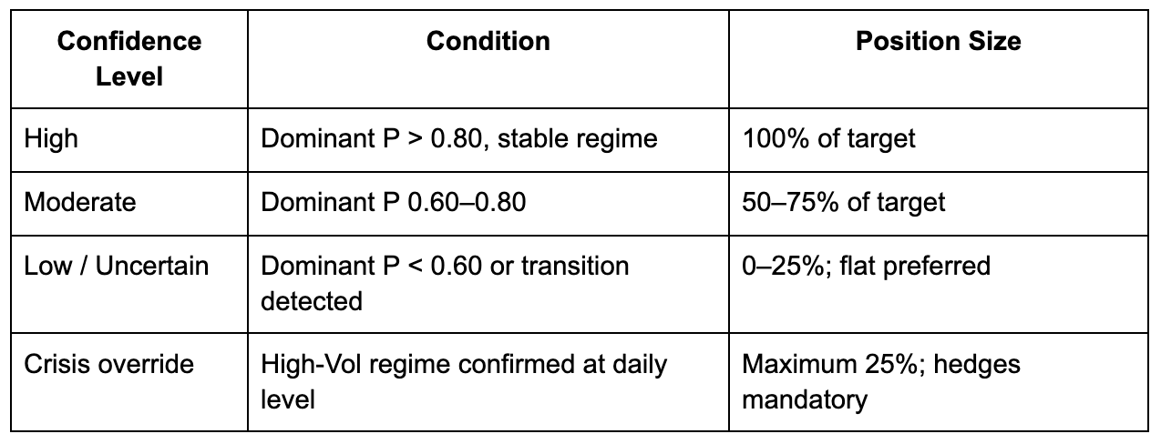
When regime confidence deteriorates, the framework automatically reduces risk.
Uncertainty itself becomes a valid signal.
Adaptive Risk Management
Regime-aware risk management differs from static approaches in one fundamental way: the risk parameters move with the market, not against it.
Position Sizing by Regime Confidence
Stop-Loss Adaptation
- Trending regimes favor wider ATR-based stops.
- Range regimes favor structural liquidity-based stops.
- High-volatility environments favor time-based risk exits to avoid noise-driven liquidation.
Circuit Breakers
The framework automatically reduces exposure when:
- Regime uncertainty remains elevated
- Liquidity deteriorates sharply
- Cross-asset volatility spikes
- News sentiment pressure becomes unstable
This creates a system designed not only to pursue returns, but also to survive regime transitions.
Conclusion
The framework presented here is designed to do one thing: translate the theoretical understanding of regime changes and market microstructure into a systematic, repeatable model-building process.
Each timeframe gets its own model, tuned to the drivers that actually govern behavior at that resolution. Those models are connected through the cross-timeframe alignment mechanism, so lower-timeframe signals are always evaluated in the context of the macro regime. And the entire system operates with explicit uncertainty quantification — when the model doesn’t know, it says so, and position sizing reflects that.
The goal is not prediction. It is regime-aware adaptation: recognize the current market state as accurately as possible, size positions proportionally to confidence, and transition gracefully when conditions change.
Traders who internalize the microstructure dynamics from the previous article and apply the model-building framework from this one have the foundation for a genuinely adaptive trading system — one that does not fight the market’s current nature, but works with it.
This article is the second in our series on regime changes and market microstructure. You can read the foundational piece – covering how regimes manifest in order flow, liquidity, and price dynamics across timeframes – here: Regime Changes and Market Microstructure.