Regime Changes and Market Microstructure

Problem Description

Many of us, at some point during our analysis of cryptocurrency market returns, have asked ourselves: what is the true nature of this data, and what lies behind the patterns we observe?
I often ask myself this same question when studying regime changes in the crypto market.

We must acknowledge that the ongoing institutionalization of crypto is a reality. The connections between crypto markets and traditional financial systems are becoming increasingly tight due to liquidity transfers and cross-market capital flows.
Some investors choose to diversify their portfolios with digital assets, seeking the opportunities they offer for significant gains.

However, we must also make an important distinction between the nature of the crypto market and that of traditional markets.
To illustrate this, imagine a football (soccer) match:

1. The referees are the regulators,
2. The players are the market participants, and
3. The ball represents the traded assets.

In traditional financial markets, the ball is round — its movement is relatively predictable within established rules.
In the crypto market, however, the ball is not perfectly round, it’s squarer in nature. This means its trajectory is harder to predict, and the dynamics of play are much less stable. The same basic rules apply, but the outcomes can differ dramatically.

This article does not claim to provide all the answers. Its purpose is to raise questions and explore opportunities to better understand one key idea:

Is there a distinct microstructure behind the regime changes in market returns?

The goal is to provoke thought and encourage discussion about the hidden structures in crypto market data.
And, as with any analysis, the validity of the ideas presented here ultimately depends on the critical review of the reader.

Now, we’ve mentioned regime changes — we already know that markets often show strong performance in October and in the first months of a new year.
But let’s go further:
What if market behavior changes not only across months, but also between days of the week and even across hours of the day?

Methodological Setup

To illustrate this concept, we use a univariate (price return) probability density function (PDF) and a model that automatically identifies the most appropriate distribution for the data.
Our working hypothesis assumes a Gaussian form; however, in practice, price returns are rarely normally distributed, especially in crypto markets where heavy tails and volatility clustering dominate. As in most cases we only assume that it is normally distributed.

For this study, we analyze two months of 1-hour BTC, AVAX, and OP price returns against USDC.

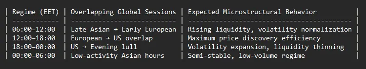
All time-based analyses are expressed in Eastern European Time (EET), which provides a regionally aligned view of intraday regime changes relative to global liquidity cycles.

These three markets were chosen randomly, ensuring no bias regarding which asset might produce stronger or weaker results.

The 1-hour granularity allows us to capture intraday market structure while maintaining sufficient data coverage for reliable statistical inference.

This timeframe strikes a balance between high-frequency sensitivity and macro-pattern observability, making it suitable for analyzing microstructural regime transitions over multi-week periods.

Weekday vs. Weekend Regime Analysis (EET context)

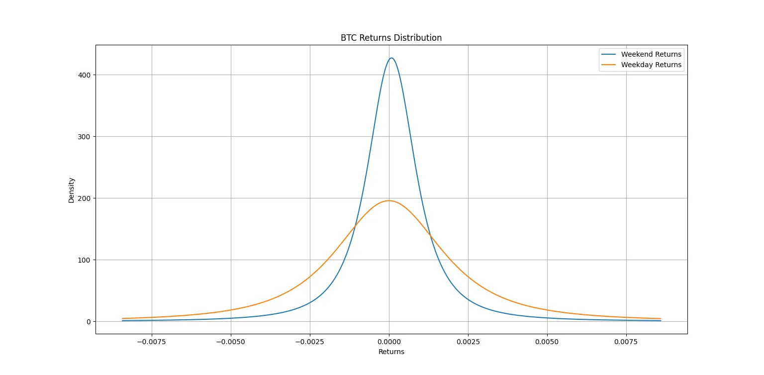
• BTC/USDC

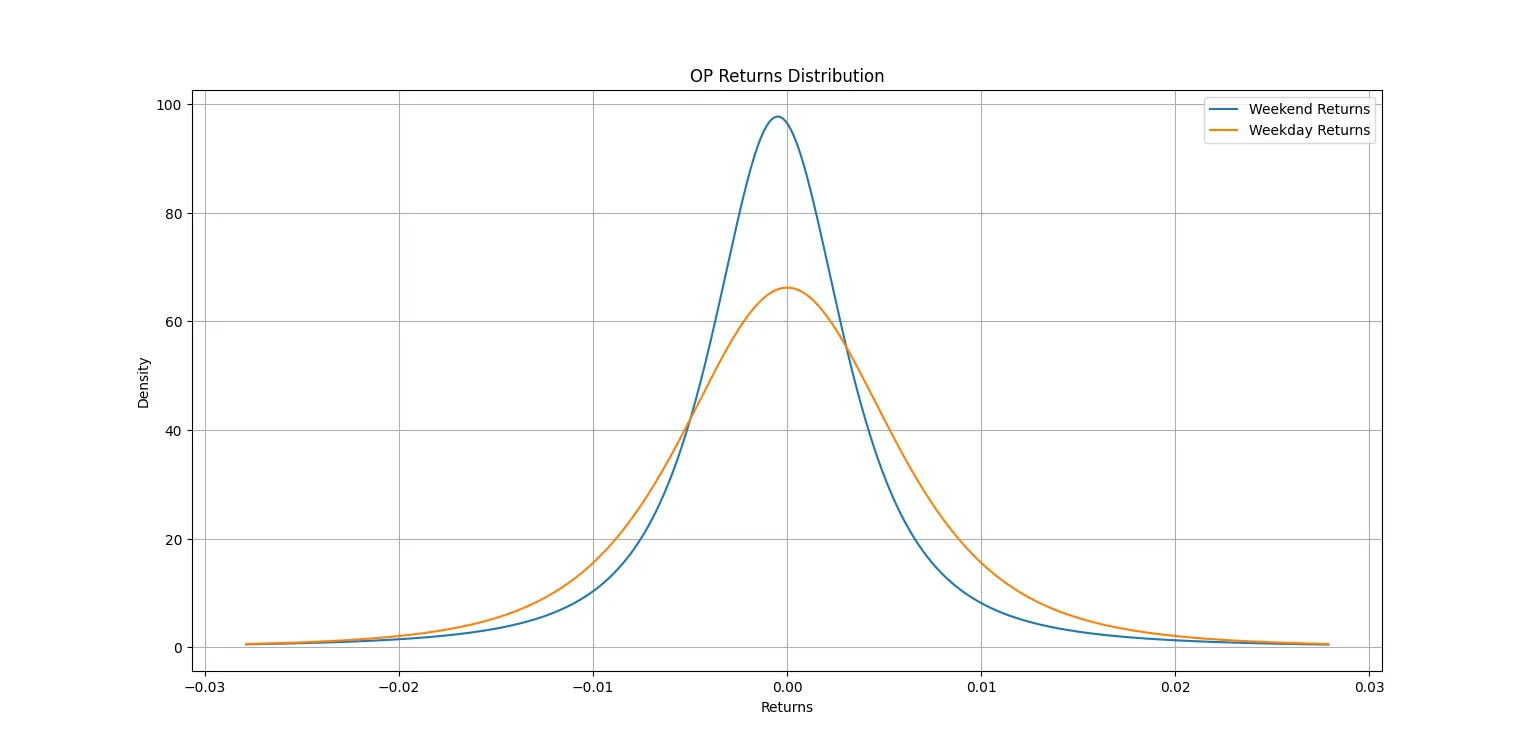
• OP/USDC

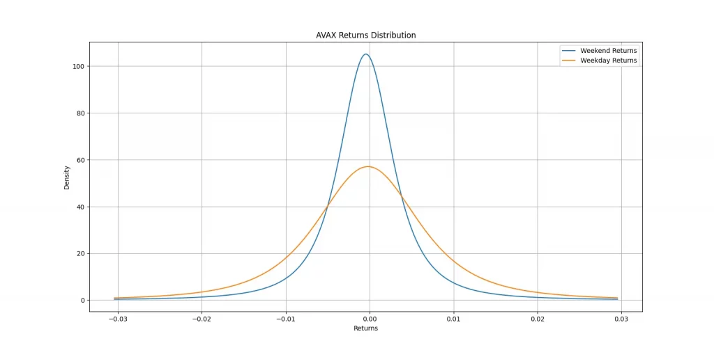
• AVAX/USDC

1. Overview of the charts

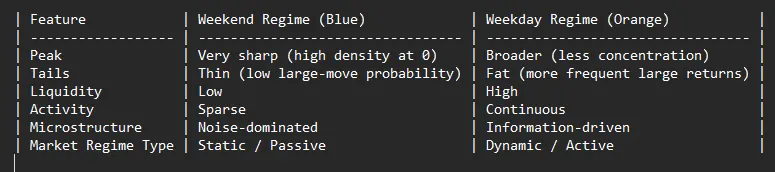
• Blue curve (Weekend Returns): Extremely peaked at zero with much thinner tails.
• Orange curve (Weekday Returns): Flatter peak and fatter tails.

This suggests that weekend returns are more concentrated near zero, while weekday returns show higher dispersion (volatility).

2. Key Observations

A. Liquidity and Volatility Regimes

• – Weekend:
  – The sharp peak indicates that price changes are small and infrequent.
  – This reflects low trading activity and thin liquidity during weekends.
  – With fewer active market participants and thinner order books, large trades are rare — leading to micro-price stability around equilibrium.
  – When moves do occur, they’re often due to exogenous news shocks rather than endogenous trading flows.
• Weekday:
  – The broader, flatter curve implies more heterogeneous returns, i.e., both small and large moves are more frequent.
  – Reflects active trading sessions, deeper liquidity, and continuous order book adjustments by market makers and algorithms.
  – This behavior matches the normal microstructure regime of major exchanges when institutional and algorithmic participants dominate flow.

B. Market Microstructure Noise and Price Discovery

• The higher density around zero on weekends means microstructure noise (bid–ask bounce, spread-induced returns) dominates actual price discovery.
• The weekday regime has more genuine price discovery due to active arbitrage and liquidity provision.

In microstructural terms:

• Weekend market: Noise-dominated, illiquid, quasi-stationary regime.
• Weekday market: Information-driven, liquid, high-turnover regime.

C. Tail Behavior and Risk

• Fat tails (weekday) → higher probability of larger returns → reflects microstructural volatility clustering (intraday volume bursts, momentum ignition, etc.).
• Thin tails (weekend) → suggests suppressed volatility and less extreme order flow imbalance.

This confirms that volatility and liquidity regimes are time-dependent, aligning with known patterns in crypto markets:

Volatility compresses on weekends and expands during trading hours of traditional financial centers (Monday–Friday overlap).

3. Summary Conclusion

Some might argue that the observed difference between weekend and weekday return distributions is partly due to the disproportionate number of weekday observations within a typical month.

To control for this and better isolate genuine behavioral effects, we can next examine the return distributions across hourly regimes, which provides a more granular view of how market microstructure evolves over time.

Hour’s regimes analysis

• BTC/USDC

• OP/USDC

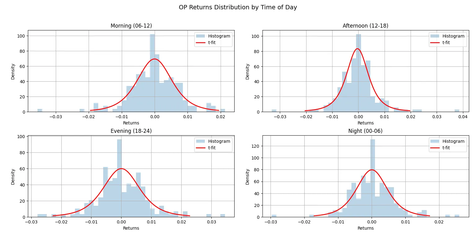
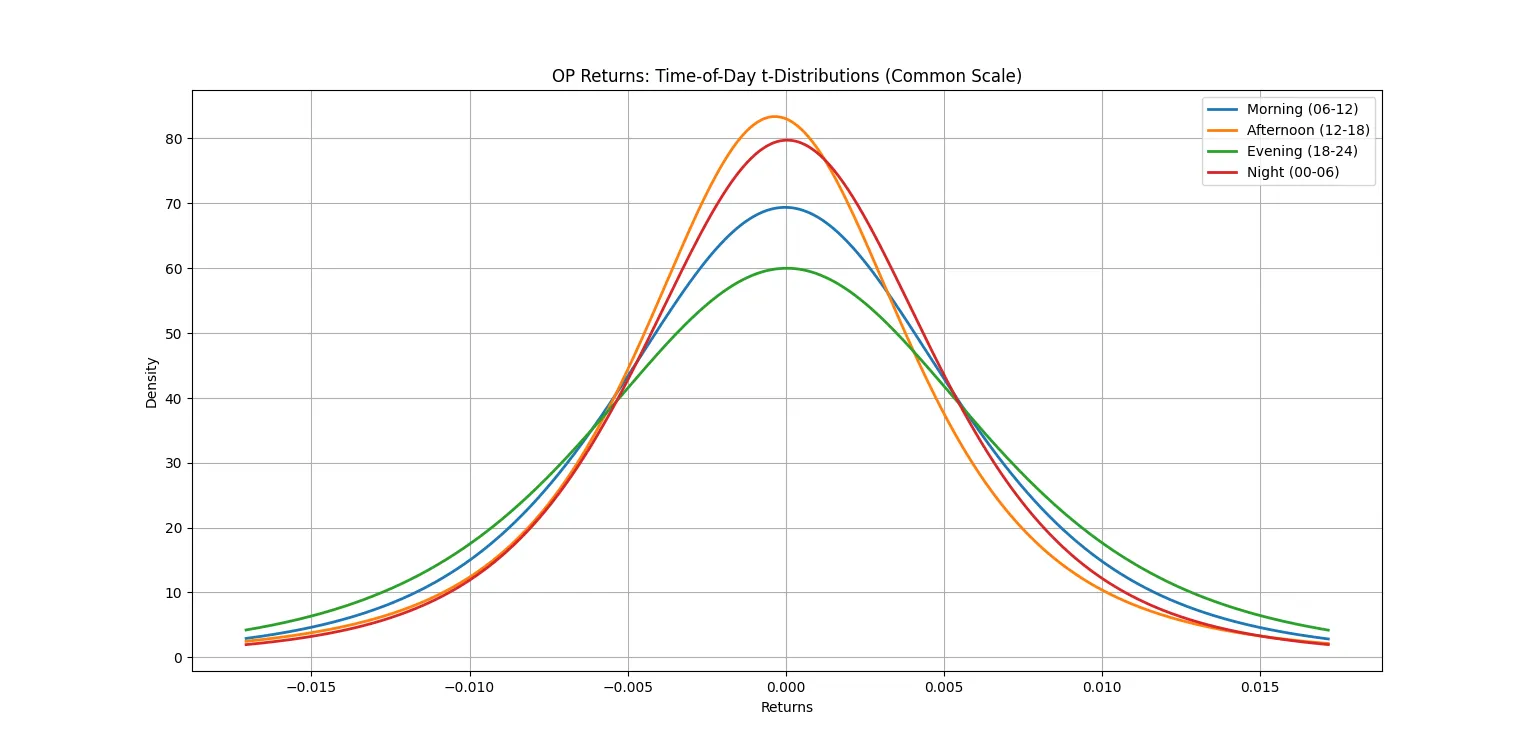
• AVAX/USDC

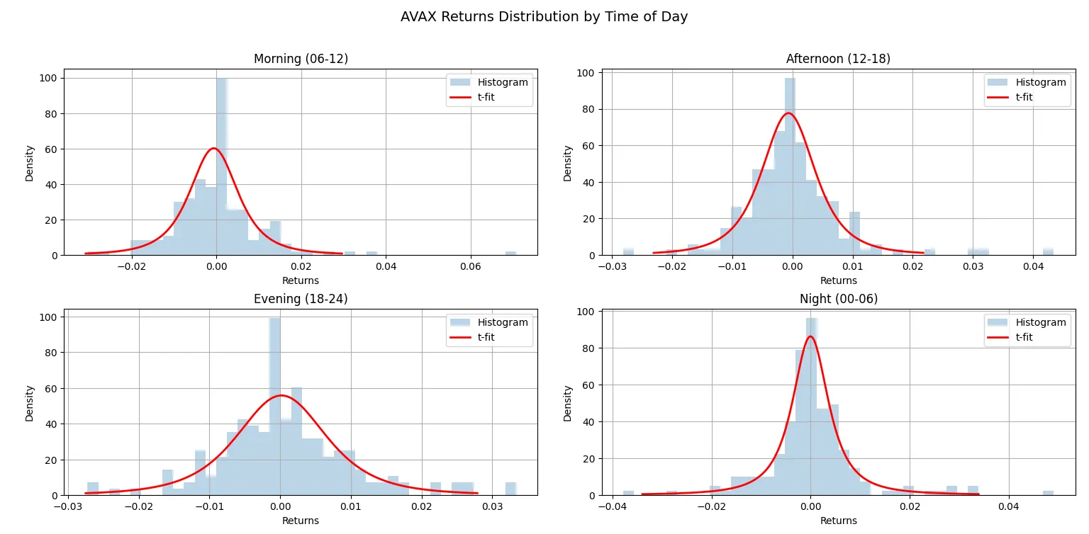
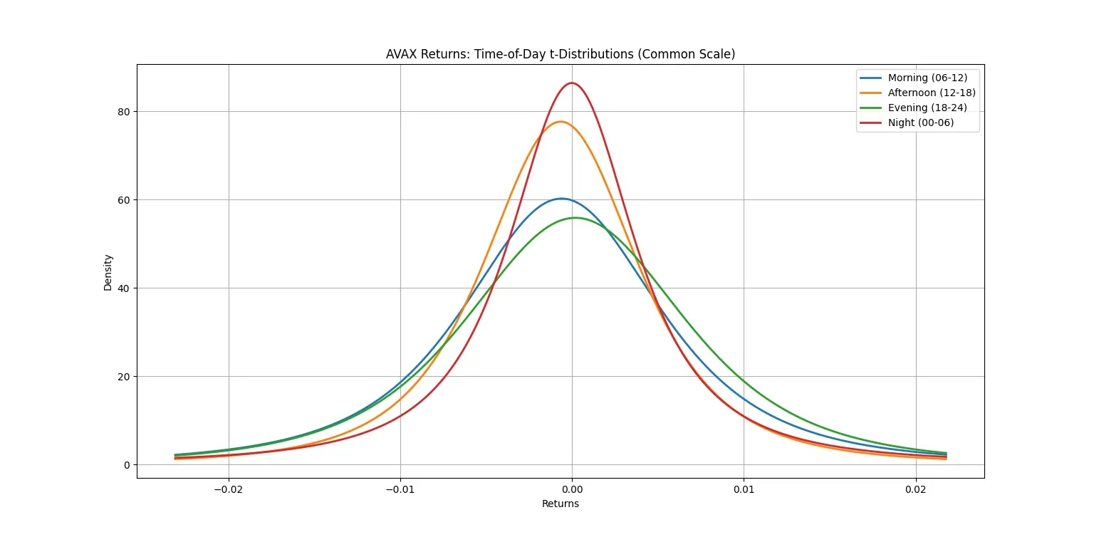
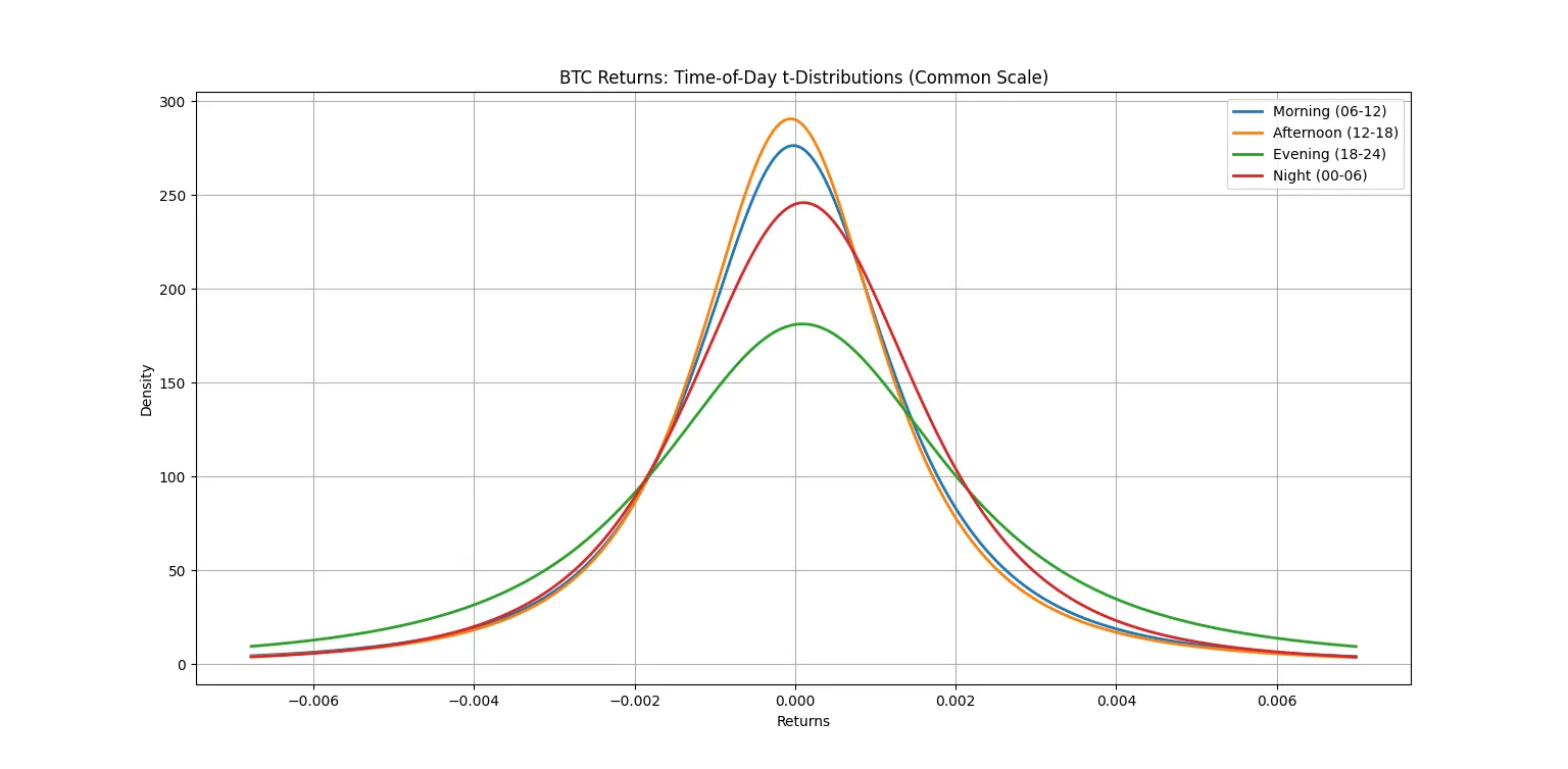
1. Overview of the chart

2. Key Observations

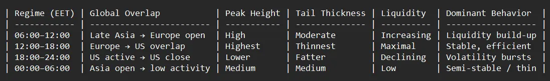
A. Intraday Volatility Regime Structure

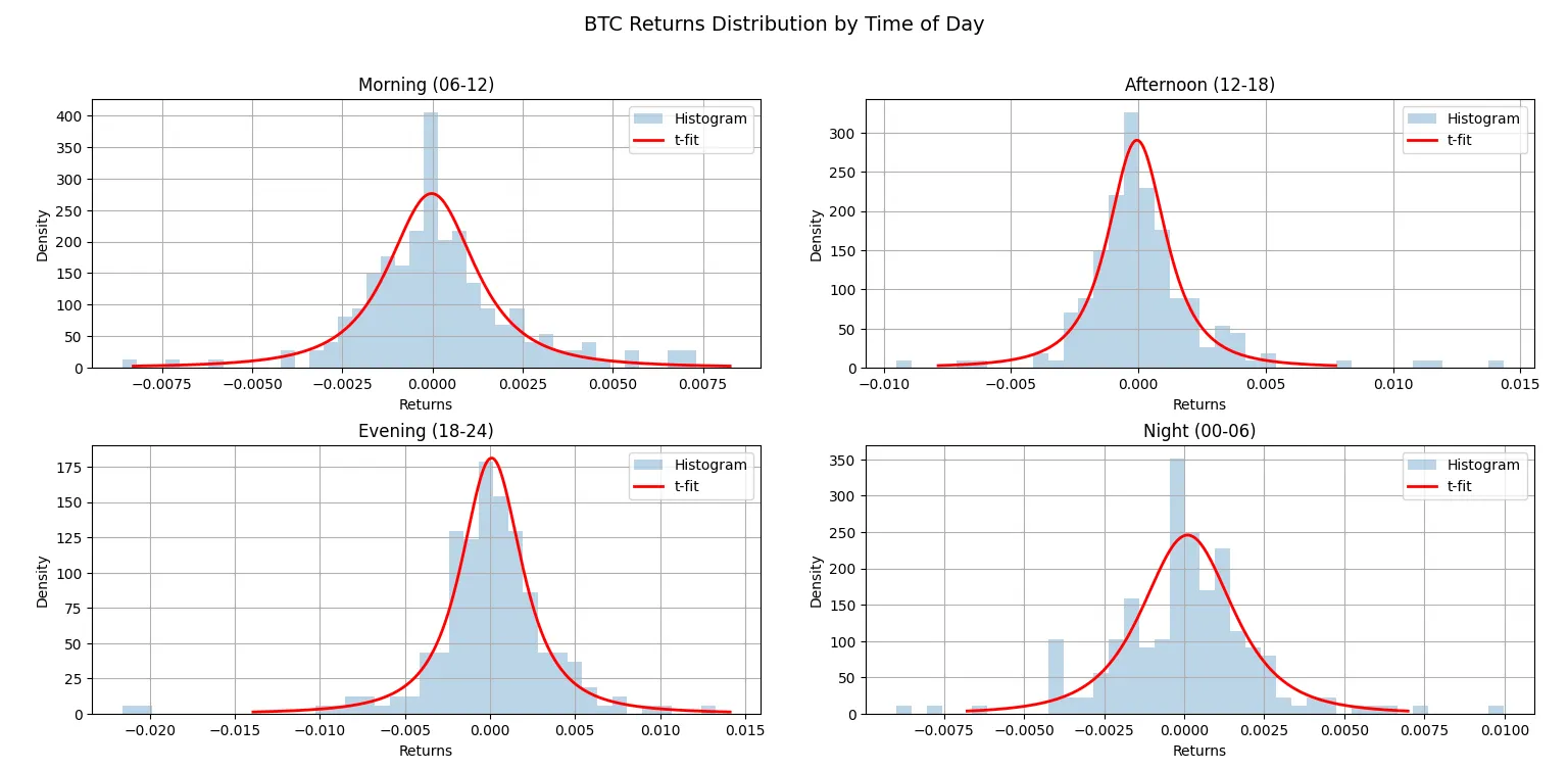
• Morning (06–12 EET):
  The distribution is relatively concentrated around zero but slightly broader than early-morning Asia.
  – Reflects the transition from thin Asian liquidity to the start of European participation.
  – Small increases in volatility and bid–ask activity as European markets warm up.
• Afternoon (12–18 EET):
  This period shows the tightest, most efficient distribution.
  – Corresponds to the Europe–US overlap, when global liquidity peaks and price discovery is most efficient.
  – Reflects strong institutional flow, algorithmic arbitrage, and deep order books.
• Evening (18–24 EET):
  The distribution widens noticeably, with fatter tails.
  – Marks the US session and its close, where volume spikes but order-book depth begins to decline.
  – Characterized by event-driven volatility and liquidity thinning after 22:00 EET.
• Night (00–06 EET):
  A moderate peak with medium tails.
  – Represents the lowest global liquidity period, dominated by Asia-Pacific markets.
  – Volatility remains relatively contained but can show sporadic jumps on regional news or thin order flow.

B. Information vs. Noise Regimes

• Morning & Afternoon (06–18 EET) → Information-driven regimes
  – High liquidity, continuous price discovery, efficient spreads.
  – Dominated by European and transatlantic institutional activity.
• Evening & Night (18–06 EET) → Liquidity-driven regimes
  – Declining order book depth, elevated price impact per trade.
  – More noise-dominated with episodic volatility bursts.

C. Temporal Asymmetry and Regime Transitions

The transition from Afternoon → Evening → Night likely represents:

• A shift from liquid to illiquid microstructure,
• A regime change where the market transitions from “informational efficiency” to “microstructure noise dominance.”

This transition is key for intraday modeling — it explains why volatility and return clustering appear around session boundaries.

3. Microstructure Interpretation

• Morning and afternoon periods (06–18 EET) represent efficient price discovery regimes.
  Bid–ask spreads are tight, and volatility is structurally dampened by the depth of liquidity.
• Evening and night periods (18–06 EET) reflect illiquid or semi-fragmented regimes,
  characterized by fatter distribution tails, indicating greater vulnerability to order-book shocks and higher short-term kurtosis.

Thus, the market microstructure alternates between two dominant intraday states:

• High-liquidity equilibrium regime (06–18 EET) — stable, information-driven trading.
• Low-liquidity transition regime (18–06 EET) — thin liquidity, noise-dominated volatility

3. Summary Conclusion

Final Conclusion: Market Microstructure Regimes

The comparison of weekday vs. weekend and hourly return distributions reveals a clear temporal segmentation of the market’s microstructure.

During weekdays, the return distributions exhibit broader shapes with fatter tails — a hallmark of active price discovery, deeper liquidity, and higher participation from institutional and algorithmic traders.
In contrast, weekends display sharply peaked, low-volatility profiles, reflecting a thin-liquidity, noise-dominated regime where price changes are infrequent and largely random.

When we shift to an hourly perspective, this regime differentiation becomes even more granular.
The morning and afternoon periods (06–18 EET) align with global trading session overlaps and show narrow, concentrated PDFs, indicating stable and efficient price formation.
Conversely, the evening and night periods (18–06 EET) demonstrate flatter peaks and fatter tails, revealing microstructural fragility — reduced liquidity depth, higher price impact per trade, and increased volatility clustering.

Taken together, these results suggest that market return dynamics are not homogeneous through time, but instead alternate between information-driven and liquidity-driven regimes.
This intraday and interday structure implies that market efficiency fluctuates with global trading activity, providing a quantifiable framework for timing-sensitive trading strategies and regime-adaptive modeling within analytical systems.