Portfolio Management using PDF and CDF

Portfolio management is the process of strategically selecting and managing a mix of financial assets—such as stocks, bonds, and other instruments—with the goal of balancing risk and return. Effective portfolio management requires more than evaluating individual assets in isolation. It involves understanding how assets behave in combination, especially during periods of market stress.

One of the key challenges in managing multi-asset portfolios is accounting for how different assets move together, a concept known as correlation or co-movement. This is where joint distribution (PDF and CDF) analysis becomes essential. By modeling the joint behavior of asset returns, portfolio managers can more accurately measure portfolio risk, identify diversification opportunities, and build more resilient investment strategies.

1. Estimating the Probability of Losses

Use Case:
Compute the probability that a portfolio loses more than a threshold amount.

Example:
Suppose daily returns of a portfolio are modeled as normally distributed:

• Mean return (μ) = 0.1%
• Standard deviation (σ) = 2%

You want to find the probability of a daily return worse than -3%.

Steps:

• Standardize the return:

• Use the CDF of the standard normal distribution (Φ):

So, there’s ~6.06% chance the portfolio loses more than 3% in a day.

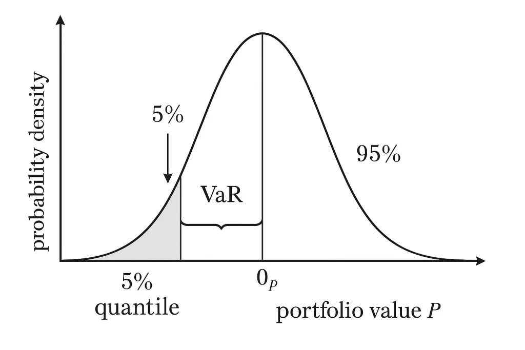
• The PDF (bell curve) shows the shape of returns;
• The CDF gives cumulative probability up to any value.

2. Calculating Value-at-Risk (VaR)

VaR indicates how much a portfolio might lose at a given confidence level.

Example:
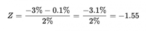
Find the 95% daily VaR.

• Look up the quantile in the standard normal distribution for 5% tail:

• Calculate the return threshold:

So, 95% of the time, losses should not exceed -3.19%.

Role of PDF/CDF:

• PDF: tells the density at each return level.
• CDF: helps find quantiles directly.

Join us now!

Start your automated trading bots.

Let's Start

3. Stress Testing and Scenario Analysis

Suppose you want to know how bad a “worst-case” market drop might be.

Example:
You simulate returns and build an empirical distribution from historical data.

• Use the empirical CDF to find the 1st percentile.
• Alternatively, fit a parametric PDF (e.g., t-distribution for fat tails) and integrate to get the CDF.

Outcome:
Determine loss levels under rare scenarios.

4. Portfolio Optimization under Downside Risk

Traditional mean-variance optimization minimizes variance. Investors might prefer minimizing downside risk (e.g. Conditional VaR).

Example:
Compute Expected Shortfall (ES) at 95% confidence:

• Calculate VaR at 95%.
• Integrate the PDF left of VaR to find the expected loss in the tail.

Mathematically:

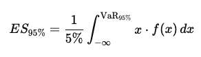
Where f(x) is the PDF of returns.

5. Joint Distribution Risk Analysis in Multi-Asset Portfolios

When analyzing multi-asset portfolios, it’s important to consider how assets move together. This is captured by the joint distribution of asset returns.

Joint Probability Density Function (PDF)

The joint PDF, denoted f(x,y), shows the likelihood of different return combinations for two assets — for example, Stock A and Stock B;

• The 3D surface plot illustrates the joint normal distribution of the two returns;
• The peak represents the most likely combination (usually around 0% return if centered);
• The shaded red region on the base represents the tail risk area, where both returns are less than or equal to –5%;
• This region helps assess the probability of a simultaneous drop in both assets;
• The PDF plot helps portfolio managers understand how likely each return combination is;

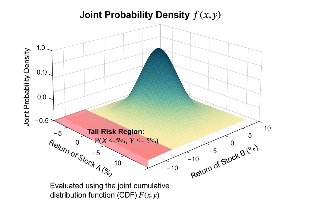
The PDF plot shows how likely different combinations of asset returns are, highlighting areas of joint tail risk such as simultaneous losses.

Joint Cumulative Distribution Function (CDF)

The joint CDF, denoted F(x,y), gives the total probability that both asset returns fall below specified thresholds;

• The contour plot shows cumulative probability increasing from the bottom-left to the top-right;
• The blue shaded region highlights the area where both Stock A and Stock B have returns ≤ –5%;
• The evaluation point at (–5%, –5%) marks where we compute the joint probability of underperformance;
• This value quantifies the risk of a joint crash or co-movement in losses;
• The CDF plot helps understand the total probability that asset returns fall below specific thresholds;

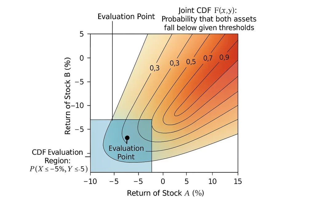
The CDF plot shows how much cumulative risk lies in regions of joint underperformance.

Why It Matters in Portfolio Management

Understanding joint distributions is essential for managing multi-asset portfolios effectively. Tools like the joint PDF and joint CDF support critical tasks such as:

1. Risk measurement (e.g., VaR, Expected Shortfall)
2. Scenario analysis for joint movements of asset returns
3. Stress testing under adverse market conditions
4. Optimization focused on minimizing downside or correlated ris
5. Tail risk estimation in multi-asset contexts

The joint PDF and CDF are fundamental to probability-based decision making in modern portfolio management, helping quantify co-movement, diversification effects, and the likelihood of simultaneous losses.