ARIMA vs ARCH models in time series analysis: guide & Python

Modern time series analysis relies on statistical models that capture various patterns in data. Two powerful models widely used in finance and economic forecasting are:

ARIMA models → focused on modeling the mean or predictable part of returns.
ARCH models → focused on modeling volatility, i.e. the variability in returns.

In this article, we’ll explore:

The general concept of ARIMA models and their variations.
The general concept of ARCH models and their variations.
Fundamental ideas like stationarity and seasonality.
Simple Python code examples.

What are stationary and seasonal data?

Stationary data have a constant mean and variance over time. They do not exhibit persistent trends or recurring seasonal patterns. Many statistical models, like ARIMA, require stationary data.
Seasonal data show regular, repeating patterns over specific intervals (e.g. months, quarters). For example, ice cream sales often spike every summer.

When seasonality is present, the data are typically non-stationary. To model them effectively, seasonal effects must be removed—e.g. through seasonal differencing or models like SARIMA.

General concept of ARIMA models and their variations

What is ARIMA?

ARIMA stands for:

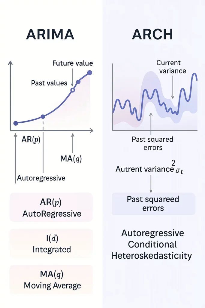
AutoRegressive (AR) – the series depends on its own past values.
Integrated (I) – differencing is applied to achieve stationarity.
Moving Average (MA) – the series depends on past forecast errors.

ARIMA models the mean of the time series by capturing:

✅ Correlation dependencies in returns (e.g. past returns help predict future values)
✅ Correlation dependencies in residuals (errors may also show patterns)
✅ No seasonality in standard ARIMA.
✅ Data must be stationary.

SARIMA: Adding Seasonality

When data exhibits clear seasonality, ARIMA extends to SARIMA (Seasonal ARIMA), which includes seasonal components to capture repeating patterns.

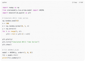
Simple ARIMA Example in Python

General concept of ARCH models and their variations

What is ARCH?

ARCH stands for:

AutoRegressive (AR) – the series depends on its own past values.
Conditional (C) – variance evolves based on past information.
Heteroskedasticity (H) – variance is not constant over time.

While ARIMA models the mean, ARCH models the volatility of the residuals left over from the ARIMA model.

ARCH captures:

✅ Heteroskedasticity → the variance changes over time rather than remaining constant.
✅ Volatility clustering → periods of high volatility tend to follow high volatility.

ARCH is extremely useful for financial data, where volatility is not constant.

Model Extensions.

GARCH (Generalized Autoregressive Conditional Heteroskedasticity)

GARCH extends the ARCH model by allowing the current volatility to depend not only on past squared errors (the ARCH effect) but also on its own past values (the GARCH effect). This results in a more flexible and realistic modeling of volatility dynamics, especially in financial time series

TARCH (Threshold Autoregressive Conditional Heteroskedasticity)

TARCH introduces asymmetry into volatility modeling, allowing negative shocks (bad news) to have a larger impact on future volatility than positive shocks of the same magnitude. This helps capture the leverage effect observed in financial markets

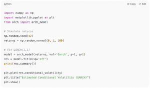
Simple GARCH Example in Python

ARIMA vs ARCH – Quick Comparison

ARIMA → Mean

Models autocorrelation in the time series.
Assumes constant volatility (unless combined with ARCH/GARCH).
No seasonality, except in SARIMA.
Data must be stationary.

ARCH → Volatility

Models heteroskedasticity (changing variance).
Captures volatility clustering.
Very useful for risk analysis and volatility forecasting.
Typically applied to residuals from an ARIMA model.

In practice, ARIMA and ARCH/GARCH are often combined:

Use ARIMA for modeling the mean.
Use ARCH or GARCH for modeling the volatility of the residuals.

Conclusion

Understanding ARIMA, SARIMA, ARCH, GARCH, TARCH, etc. helps you:

✅ Model predictable patterns in time series data (ARIMA/SARIMA).
✅ Analyze and forecast volatility (ARCH/GARCH/TARCH).

If you work with economic indicators or financial data, these models are fundamental tools for high-quality forecasting.

Curios to find out more about AIC and BIC.

ARIMA and ARCH models in time series analysis: guide & Python