One of the most fundamental ideas in data science and analytics is data distribution. It is a very important concept that helps analysts know how data is distributed, which further impacts statistical analysis, decision-making, and predictive modeling.
In this blog post, we will be explaining what data distribution is, why it’s so important, and how to generate a PDF (Probability Density Function) in Python.
What is data distribution?
Data distribution is a way that values within a dataset are spread or distributed within some range. It’s the form or structure data has when it’s graphed on a chart or graph. It informs us about helpful aspects of the structure and form of the dataset that underlies.
There are many types of data distributions employed in statistics, but the most recognized are:
- Normal Distribution: Also referred to as the Gaussian distribution, it’s a very common distribution that is applied in statistics. It is symmetrical and bell-shaped. The majority of natural phenomena (like heights of humans, test scores, etc.) adhere to a normal distribution.
- Uniform Distribution: In this type of distribution, all outcomes are equally likely to occur. This distribution contains a flat, even value distribution over the range.
- Exponential Distribution: This is usually used to model the time gap between events in a Poisson process, such as waiting times between bus arrivals.
- Binomial Distribution: Used for data that can have two results, e.g., success or failure. This is often encountered in scenarios where there are a known number of trials with fixed probabilities.
Why it is important in data analysis?
Knowledge of the data distribution is essential since it informs us about the general structure, central tendency, and variability of data. This is why it matters:
- Why knowledge of data distribution matters: Through knowledge of the distribution of your data, you can determine if the data set follows a recognizable distribution (normal or exponential). This helps to choose the right statistical tests and modeling methods.
- Outliers’ detection: Certain distributions, such as normal distributions, are sensitive to outliers. Outliers must be detected and handled as they have the propensity to skew results and render conclusions inaccurate.
- Choosing statistical techniques: Different distributions can require the use of different statistical techniques. For example, if your data is normally distributed, you can use standard parametric tests (e.g., t-tests). If it isn’t normally distributed, non-parametric techniques (e.g., the Mann-Whitney U test) would be the preferred choice.
- Predictive modeling: For machine learning models, the distribution of data typically dictates the most appropriate algorithms for making good predictions. For instance, linear regression requires normally distributed data, whereas tree-based algorithms like Random Forests are more forgiving with data distributions.
What is a probability density function (PDF)?
A Probability Density Function (PDF) is a statistical function that characterizes the probability of a continuous random variable assuming a specific value. In continuous distributions, the probability of a variable assuming an exact value is mathematically zero, but the PDF enables us to compute the probability that the value lies within a specific interval.
Briefly speaking, a PDF helps to visualize data distribution and gives a tool to calculate probabilities. The area under the curve of the PDF is the total probability, and this should be the same at 1.
Creating your first PDF in Python
Now that we have an idea of what PDF and data distribution are, let’s generate a PDF in Python. We will generate a basic Normal Distribution PDF and plot it using libraries such as NumPy and Matplotlib.
Create a normal distribution PDF:
import numpy as np
import matplotlib.pyplot as plt
# Set mean (mu) and standard deviation (sigma)
mu, sigma = 0, 0.1
# Generate random data
data = np.random.normal(mu, sigma, 1000)
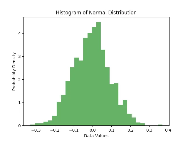
# Create histogram of the data
plt.hist(data, bins=30, density=True, alpha=0.6, color='g')
plt.title('Histogram of Normal Distribution')
plt.xlabel('Data Values')
plt.ylabel('Probability Density')
plt.show()
Create the PDF Curve:
Now, let’s calculate the Probability Density Function (PDF) for the normal distribution and overlay it on the histogram.
from scipy.stats import norm
import numpy as np
import matplotlib.pyplot as plt

# Example data
data = np.random.normal(loc=0, scale=1, size=1000)
mu, sigma = np.mean(data), np.std(data)

# Plot histogram first
plt.hist(data, bins=30, density=True, alpha=0.6, color='b')

# Get the actual x-limits after histogram is drawn
xmin, xmax = plt.xlim()
x = np.linspace(xmin, xmax, 100)
p = norm.pdf(x, mu, sigma)

# Plot the PDF
plt.plot(x, p, 'k', linewidth=2)
plt.title('Histogram and PDF of Normal Distribution')
plt.xlabel('Data Value')
plt.ylabel('Probability Density')
plt.show()
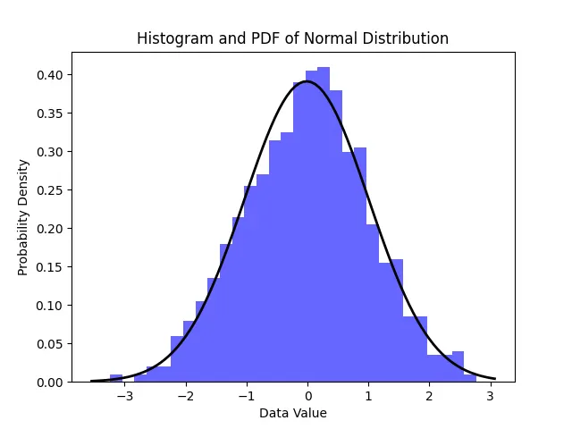
Histogram with PDF plot
Understanding data distribution is one of the pillars of data analysis. It enables you to make sense of your data, identify trends, outliers, and make informed decisions regarding the behavior of the data. In this post, we have understood the basics of data distribution, the importance of PDF in data analysis, and even built a simple normal distribution PDF in Python.
Data analysts and scientists need to visualize and analyze data distributions. With Python’s powerful libraries, you can easily create and visualize these distributions, which are essential in comprehending the underlying trends in your data.