Statistically working, either with finance or data analysis, two of the biggest terms that are always brought up are the Probability Density Function (PDF) and the Cumulative Distribution Function (CDF). Understanding what is the principal difference between PDF and CDF is essential, especially in use cases where portfolio management is concerned, with key decisions relying on risk and return distributions.
What is the principal difference between PDF and CDF?
- Probability Density Function (PDF) is the manner in which probability is distributed over a value of a continuous random variable. It shows the relative likelihood for the variable to take on a specific value.
- Cumulative Distribution Function (CDF) gives the total probability that a random variable has a value less than or equal to some specific point. It’s essentially just the total of probabilities up to this point.
Briefly:
- PDF answers: How likely is a specific value?
- CDF answers: How likely is it that the value is less than or equal to X?
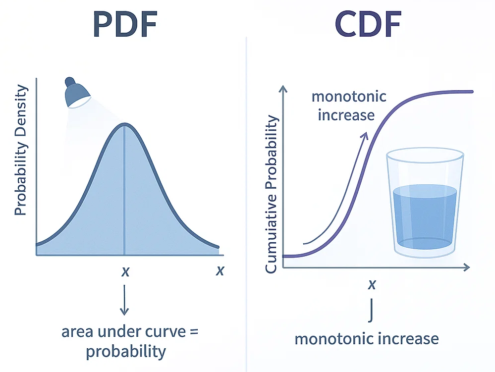
PDF vs. CDF – Visualization
- The PDF graph will have peaks where certain values are more probable. The area under the whole PDF graph will be 1.
- The CDF graph will start at zero and rise to one, showing cumulative probability. The CDF is always non-decreasing.
Use case scenarios in portfolio management
Identification of PDFs and CDFs is very important in portfolio management, particularly in risk analysis, asset allocation, and measuring performance. Let us discuss some illustrations.
1. Risk assessment
PDF Application:
- A portfolio manager analyzes the PDF of the returns of assets to find out the most likely values of return and the spread (volatility).
- For instance, if the PDF is narrow, it represents stable returns, but if it is wide, then it indicates high risk.
CDF Application:
- Managers use the CDF to approximate probabilities of losses or gains above some thresholds (e.g., the chance that returns are less than -5%).
2. Value at risk (VaR) calculation
- The CDF helps estimate the Value at Risk by determining the point at which a given percentage of worst-case losses lie.
- Example: A manager may decide that there’s a 5% chance the portfolio loses more than $1 million in a day.
3. Stress testing and scenario analysis
- PDFs are applied to scenario simulation through the representation of the likelihood of different outcomes.
- CDFs subsequently quantify the likelihood that cumulative gains or losses stay within tolerable bounds when subjected to stress
4. Asset allocation decisions
- By comparing the PDFs of different assets, one can spot combinations whose return distributions are advantageous.
- CDFs enable managers to compute the probability that the overall portfolio return will be greater than a target amount.

Start your automated trading now!

Conclusion
In general, the main difference between PDF and CDF is how they convey probabilities. The PDF tells us how probabilities are measured for specific values, while the CDF adds those probabilities up through to a specific point. Portfolio management can utilize both utilities to great advantage in measuring and controlling risk, optimizing asset allocation, and making informed investment choices.
Understanding these concepts enables professionals to navigate uncertainty, guard investments, and attain financial goals with greater certainty.