Hurst Exponent as a Statistical Test for Mean Reversion in Financial Time Series

Before developing any profitable trading, forecasting, or signal-processing strategy, the analyst must first identify the fundamental nature of the data: whether the time series is mean-reverting, purely random (random walk), or exhibits persistence (trending). The Hurst exponent (H), named after the British hydrologist Harold Edwin Hurst, is a statistical measure used to quantify the “long-term memory” of a time series. It is an essential tool for traders and researchers focused on the development of mean-reversion strategies.

It is important to note that the Hurst exponent measures long-term dependence rather than short-term autocorrelation and does not constitute a direct trading entry signal.

1. Definition and Mathematical Foundation

The Hurst exponent is defined through the asymptotic behavior of the so-called rescaled range as a function of the observation window length. The mathematical relationship follows a power-law form:

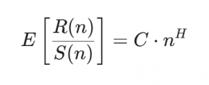
where:

• E[x] – Expected value of the statistic
  
• R(n) – Range of the first n cumulative deviations from the mean
  
• S(n) – Standard deviation of the first n observations
  
• n – Number of data points in the observation window
  
• C – Constant
  
• H – Hurst exponent

In practice, H is estimated by taking the logarithm of both sides of the equation:

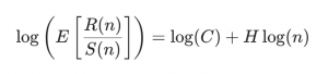
For different window lengths nnn, we compute R(n)/S(n) and average it for each given n. We then apply a logarithmic transformation.

This implies that if we define:

X = log(n)

Y = log(E [ R(n) / S(n) ])

An approximately linear relationship exists between X and Y. By plotting the points (X,Y) for all selected values of nnn, a linear regression of the form:

Y = a + bX

The slope b corresponds to the Hurst exponent H.

2. Interpretation of Results

The value of the Hurst exponent HHH lies in the interval (0,1)(0, 1)(0,1) and allows for the classification of a financial asset’s behavior into three primary market regimes:

H < 0.5: Anti-persistence (Mean Reversion)

When H<0.5H < 0.5H<0.5, the time series exhibits anti-persistent behavior, characterized by negative long-term autocorrelation. This implies that price movements tend to reverse over time—upward movements are more likely to be followed by downward movements, and vice versa.

Such a regime is typical of mean-reverting processes, where prices fluctuate around a long-term equilibrium level. The market can be described as self-correcting, without a sustained directional bias.

H = 0.5: Random Walk

A value of H≈0.5H \approx 0.5H≈0.5 indicates that the time series follows a random walk, implying the absence of long-term memory. Price movements are statistically independent and lack a predictable structure.

In this regime, price dynamics are often modeled using Brownian motion, which forms the foundation of classical financial models, including the Efficient Market Hypothesis. Past price behavior does not provide useful information about future movements.

H > 0.5: Persistence (Trending)

When H>0.5H > 0.5H>0.5, the time series displays persistent behavior, characterized by positive long-term autocorrelation. In this regime, price movements tend to continue over time—uptrends are more likely to persist than to reverse, and vice versa.

This behavior is typical of trending markets, where prices exhibit momentum and a sustained directional movement, often associated with momentum-based effects.

3. Mean Reversion and Financial Applications

The theory of mean reversion assumes that, under certain market conditions, financial variables such as stock prices or exchange rates tend to revert to their long-term average after extreme deviations. In this context, the Hurst exponent serves as a statistical filter for identifying mean-reverting regimes in financial time series.

• Identification of Opportunities

If, for example, the stock of Company X is estimated to have H=0.35H = 0.35H=0.35, this indicates strong anti-persistent behavior. Significant deviations from the average price are likely to be temporary, creating potential opportunities for mean-reversion-based strategies that aim to exploit deviations from equilibrium levels.

• Long-Term Memory

Unlike processes resembling white noise—where historical data contains no informative value—low values of the Hurst exponent reflect the presence of long-term dependence. Past price movements statistically influence future behavior, allowing for the modeling of self-correcting mechanisms.

• Examples of Consistent Strategies

• • Pairs Trading:
    The Hurst exponent can be used as a preliminary diagnostic tool when analyzing the price spread between two assets. A spread with H<0.5H < 0.5H<0.5 indicates mean-reverting behavior, which is a necessary (though not sufficient) condition for the application of pairs trading strategies.
  • Statistical Arbitrage:
    By analyzing instruments with low Hurst exponent values, analysts can identify statistically stable equilibrium states that have been temporarily disrupted by the market and construct strategies aimed at their gradual restoration.

4. Practical Implementation: Python Script for Estimating the Hurst Exponent

For practical application, established statistical libraries in Python are used. The following class enables the estimation of the Hurst exponent and the classification of market regimes:

import numpy as np
import pandas as pd
import nolds
from scipy import stats


class MarketRegimeDetector:
    """
    High-level market regime detection using
    established statistical libraries.
    """

    def __init__(self, returns, significance_level=0.05):
        self.returns = returns.dropna()
        self.alpha = significance_level

    def estimate_hurst(self):
        """Estimates the Hurst Exponent using R/S method."""
        hurst_value = nolds.hurst_rs(self.returns.values)
        return hurst_value

    def classify_market(self, hurst_value):
        """Classifies market behavior based on Hurst Exponent."""
        if hurst_value < 0.45:
            return "Mean Reverting"
        elif hurst_value > 0.55:
            return "Trending"
        else:
            return "Random Walk"
    def analyze(self):
        hurst = self.estimate_hurst()
        regime = self.classify_market(hurst)
        return {"hurst_exponent": hurst, "market_regime": regime}

Description:

• estimate_hurst() computes the Hurst exponent using a standardized R/S procedure (nolds).
• classify_market() categorizes the market as Mean Reverting, Trending, or Random Walk.
• analyze() integrates all results into a unified market regime assessment.
  

Conclusion

The Hurst exponent provides a mathematically grounded framework for assessing the potential for mean reversion in financial time series. Whether applied within an algorithmic trading model or a broader market analysis, its inclusion offers deep insight into the structural properties of the data. A well-designed strategy grounded in the Hurst exponent and supported by rigorous statistical validation can represent a source of consistent performance within an otherwise chaotic market.