Historical data is the foundation of portfolio analysis. By examining past returns, investors evaluate not only average performance but also the distribution of risks and opportunities. Traditional measures such as the Sharpe Ratio and Sortino Ratio often fall short in capturing the asymmetry and fat-tailed nature of asset returns—especially in volatile markets like crypto.
The Omega Ratio addresses this limitation by analyzing the entire return distribution, providing a more complete picture of risk-adjusted performance.
A Brief History of the Omega Ratio
The Omega Ratio was introduced in the early 2000s by Con Keating and William F. Shadwick, researchers in finance who were dissatisfied with the limitations of traditional risk-adjusted metrics. The Sharpe Ratio, for example, relies heavily on mean and variance, which assume normally distributed returns. But in reality—especially in hedge funds, alternatives, and crypto—returns are often skewed, fat-tailed, and asymmetric.
Keating and Shadwick wanted a single metric that incorporated the entire return distribution, not just averages or downside deviations. Their solution was the Omega Ratio, which elegantly frames investment performance as the balance of probabilities between good and bad outcomes relative to a chosen threshold.
They called it Omega because Omega (Ω) is the last letter of the Greek alphabet, symbolizing something final or complete. The name reflects their ambition: to provide the “ultimate” performance measure that captures everything about risk and reward in one ratio.

Create your account
Start your automated trading bots.

Definition of Omega Ratio
The Omega Ratio measures the probability-weighted ratio of returns above a given threshold to those below it.
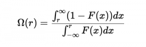
Where:
- r = threshold return (e.g., 0% or risk-free rate)
- F(x) = cumulative distribution function of returns
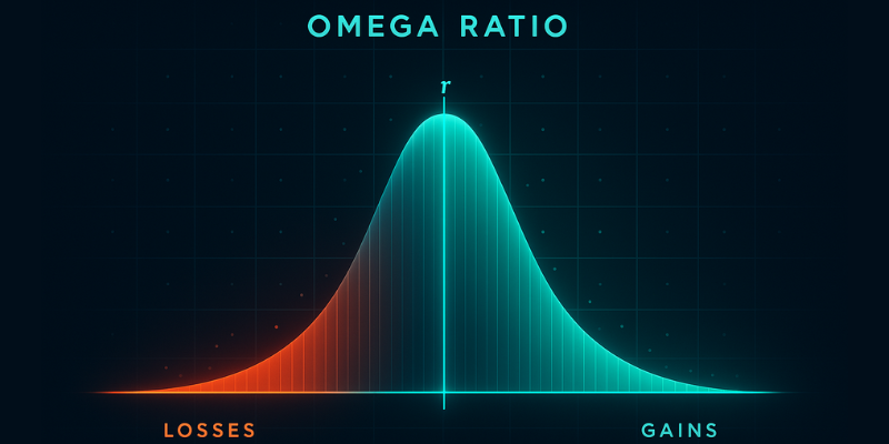
Interpretation:
- Ω > 1 → More upside potential than downside risk
- Ω < 1 → More downside risk than upside potential
- Ω = 1 → Balanced gains and losses
Python Approach: Calculating Omega Ratio
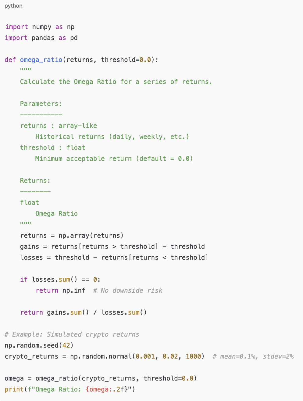
Explanation of Code
- We create synthetic history via Normal-distributed daily log returns as a baseline; heavier-tailed models (e.g., Student’s t) may be more realistic
- Define a threshold – in most cases, 0% (break-even) or the risk-free rate.
- Calculate gains and losses relative to threshold.
- Return ratio of total gains to total losses.
Sample Output
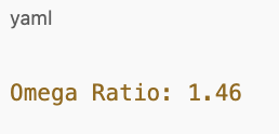
This means that the strategy delivers 1.46 units of upside potential for every 1 unit of downside risk.
Use Case Scenario
Imagine you are evaluating two trading strategies for Ethereum:
- Strategy A has a Sharpe Ratio of 0.9 and an Omega Ratio of 1.3.
- Strategy B has a Sharpe Ratio of 0.9 but an Omega Ratio of 1.8.
Although both look equal under Sharpe, Strategy B clearly offers more upside relative to downside, making Omega Ratio the better tool for decision-making in volatile crypto environments.
With this Python approach, you can extend the function to compare multiple portfolios, backtest crypto strategies, or even integrate it into automated trading bots.